FlashInfer Autotuner v2: Tune the Way You Serve

Part of FlashInfer 0.7. See the release highlights for upgrade notes.

How FlashInfer rebuilt GPU kernel autotuning for better production LLM serving at scale.

Overview

FlashInfer v0.7 introduces Autotuner v2, a redesign of how FlashInfer measures, persists, and reuses GPU-kernel choices. The same operation can often run through several backends, algorithms, or configurations, which FlashInfer calls tactics. Because the fastest tactic changes with shape and GPU, the autotuner measures candidates during warmup and reuses the winner during execution.

The legacy v1 design treated GPU device time as the ranking objective. That proxy works when omitted host overhead is negligible or nearly equal across tactics, but execution mode can break the assumption. Eager execution repeats framework and backend launch work on every call; under CUDA Graph execution, the launch sequence is captured once, so tuning ranks replay latency. The legacy cache did not record that distinction as an explicit policy.

For example, on NVIDIA Blackwell (SM100), a measured bmm_fp8 cuDNN candidate at $M=8$ and $N=K=8192$ took about 8 microseconds (µs) when timing excluded host work, but about 330 µs when called repeatedly in eager mode. Because the recurring host cost varied by tactic, the device-time winner could lose the full eager call. The kernel did not change; the measurement boundary did.

Reuse adds a second system problem. A winner shared across calls, process restarts, and distributed ranks can be misapplied if its key is incomplete, become unusable as its runtime changes, or diverge across ranks. Autotuner v2 therefore treats the winner as a deployment artifact. We explain the redesign and its evidence in five parts:

1. The best tactic depends on how you run it. Eager execution includes recurring host cost; CUDA Graph execution ranks captured replay.
2. A winner is valid only in context. The environment, operation, and measurement policy determine where a saved result can be reused.
3. Cache correctness across calls, processes, and ranks. Atomic publication, optional tactic validation, in-memory promotion, and explicit rank convergence keep reused choices valid and consistent.
4. Benchmark methodology: beyond single-kernel timing. Independent oracle, selection, persistence, and multi-rank experiments separate what is measured from how each claim is tested.
5. What the benchmarks showed. The results quantify selection quality, cache cost and correctness, and rank agreement, then show where the measurements changed the implementation.

Across 276 matched eager workloads, median regret, the latency penalty relative to the measured best tactic, fell from 1.390% with v1 event timing to 0.418% with v2 eager timing. The matrix-wide mean fell from 96.08% to 0.958%, reflecting a high-regret tail in v1: the number of workloads above 100% regret fell from 59 to zero. Across 281 CUDA Graph workloads, median regret moved from 0.0565% to 0.00646%, while mean regret moved more modestly from 0.346% to 0.215%. In four B200 and GB300 configurations, steady-state v2 lookup latency stayed within 0.72% of v1, with zero filesystem operations and zero JSON calls over 600 lookups. We evaluated 14 tuned operation surfaces across NVIDIA H100, B200, GB200, and GB300 GPUs; Figure 8 shows the measured coverage.

1. The best tactic depends on how you run it

The SM100 bmm_fp8 example makes the central requirement concrete: a useful autotuner must identify the fastest tactic under the execution mode that will actually run. Device time is an adequate proxy only when omitted host work is negligible or nearly equal across tactics.

Figure 1 summarizes the resulting design choice: eager and CUDA Graph execution expose different costs, so they can produce different winners for the same operation and environment.

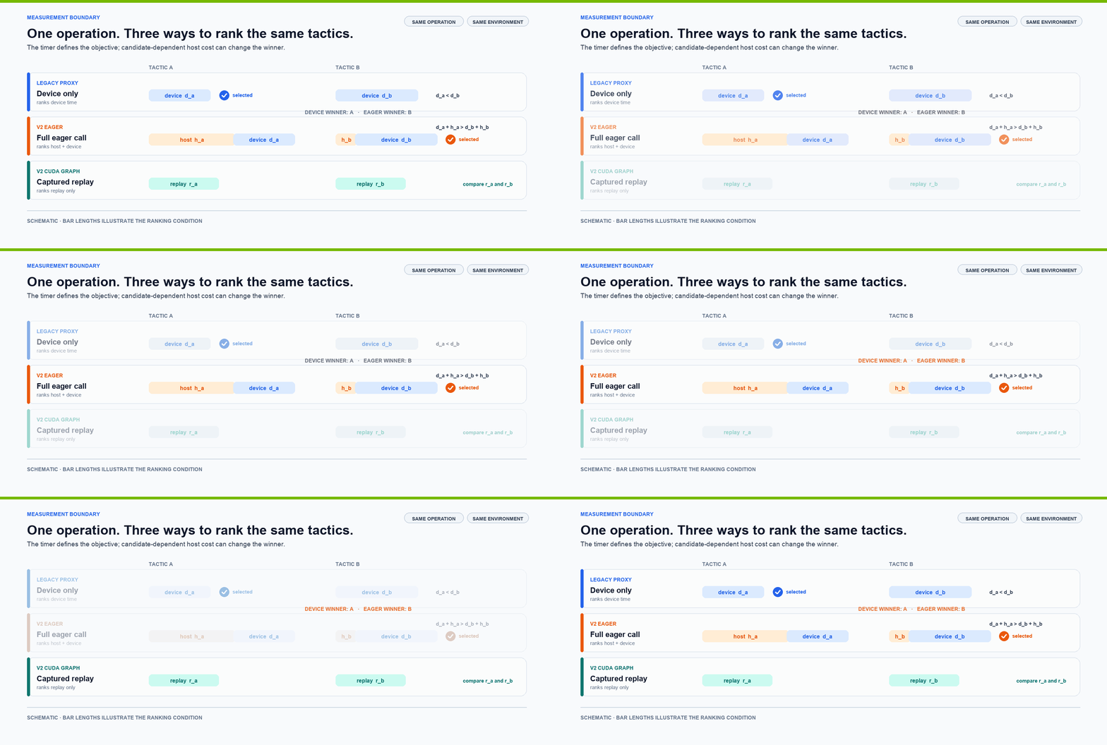
Figure 1. The measurement boundary can change which tactic wins.

Autotuner v2 therefore exposes two explicit measurement modes. Eager mode ranks the recurring call, including host and device work. CUDA Graph mode captures the operation once and ranks replay latency.

For two tactics $a$ and $b$, let $d_a$ and $d_b$ be their device times, and let $h_a$ and $h_b$ be the recurring host costs paid by eager execution. Device-only timing can prefer $a$, while the full eager call prefers $b$:

$$d_a<d_b \qquad\text{but}\qquad d_a+h_a>d_b+h_b.$$

The left inequality is the ordering seen by the legacy timer; the right is the ordering of the full eager execution path. More device-only samples can reduce noise in the measured device times, but they cannot recover omitted, candidate-dependent host cost. That is the ranking reversal seen in the bmm_fp8 example.

We designed MeasurementPolicy to carry this execution choice into tuning. There is no universally correct measurement boundary, only the one the deployment will actually run.

To avoid silently changing existing integrations, the default remains legacy-compatible. When a caller explicitly selects eager or CUDA Graph measurement, v2 records that non-default policy in the persistent environment identity, preventing a result measured for one execution mode from being reused as if it belonged to the other.

2. A winner is valid only in context

Measuring the right execution path answers how to choose a winner. Persistence introduces the next question: when can a saved answer be reused by later calls or a fresh process? The selected tactic depends on the operation, environment, and measurement policy, so v2 must preserve all three as the result’s context.

In v1, frameworks and other callers supplied much of that machinery themselves: the filename, compatibility fields, invalidation rules, and loading or broadcast of a monolithic JSON file. Different integrations naturally encoded different reuse policies. Autotuner v2 brings this artifact boundary into FlashInfer so the library that creates a tactic also defines when it can be reused.

Each result receives two levels of identity. The environment identity asks, “Can this runtime reuse the result?” It covers the cache schema, GPU, FlashInfer and CUDA versions, relevant backend and compiler versions, and any non-default measurement policy. The operation identity asks, “Is this the same tuning problem?” It combines the custom operation, runner class, resolved shape bucket, and runner-specific extras such as layout, activation, quantization, or expert structure.

The split prevents two different kinds of aliasing. Across environments, a result measured with an explicit eager policy on B200 does not share a namespace with a CUDA Graph result or one from another GPU, even when they use the same operation and shape. Within one compatible environment, runner-specific extras keep apart calls that a shape bucket alone would merge. In the GB200 key-ablation test, otherwise matched CUTLASS MoE calls with top_k=8 and top_k=4 mapped to different operation keys through extras. Without those distinctions, a well-formed file could still return a winner for a different call.

Figure 2 shows how runtime-wide fields choose the environment directory while operation-specific fields choose one entry inside it.

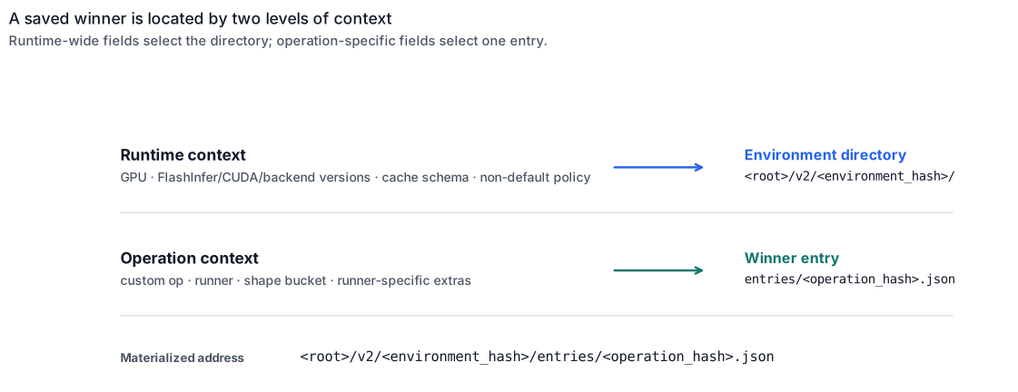
Figure 2. Compatibility selects the directory; the operation selects the entry.

The on-disk layout follows the same split. A runtime change moves lookup to another directory; an operation change selects another entry without invalidating unrelated operations.

Identity only routes a call to the intended file. Correct reuse also requires a complete entry, a tactic that remains usable for the current call, and a consistent choice across distributed ranks. The next section explains how v2 enforces those conditions.

3. Cache correctness across calls, processes, and ranks

Finding the intended cache entry is not enough to make reuse correct. A hit skips measurement, so the stored entry must be complete, its tactic must still be usable for the current call, and participating ranks must enter execution with compatible choices. Autotuner v2 handles those requirements at three boundaries: publication, acceptance, and rank convergence.

Publish a complete winner. During warmup, the tuning context attaches a managed store and profiles only misses. The normal untuned path participates as a candidate, so the published winner does not lose to the default under the same probe and measurement. v2 writes a complete per-operation entry to a temporary file in its destination directory, then installs it with an atomic rename. Concurrent processes may duplicate tuning work, but readers cannot see a half-written file, and no process needs to merge a monolithic cache at exit.

Leaving the tuning context stops profiling but keeps the store attached. Serving can read the winner from process memory. A fresh process preloads eligible winners when it attaches the same store, then promotes each one into the hot lookup cache on first use. Steady-state calls neither reopen the entry nor reparse its JSON. Figure 3 follows this lifecycle from warmup through in-memory serving and fresh-process hydration.

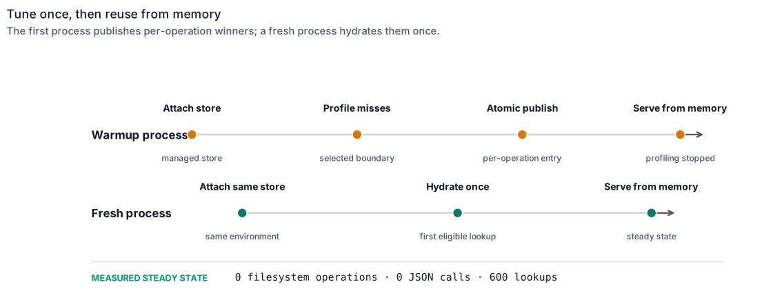
Figure 3. Tune during warmup; serve from the attached result.

Accept only a usable hit. Reaching the intended entry is not enough. Even a syntactically valid tactic can become unusable if a backend’s available plans change with library version, shape, or device. Invalid JSON, a mismatched embedded key, or an entry stored under the wrong environment must also fail closed. Autotuner v2 turns those cases into misses and lets a runner validate a loaded tactic against current inputs before reuse.

Focusing on the v2-managed path and omitting legacy and bundled cache sources, the decision flow can be summarized in Python-like pseudocode:

namespace = environment_id(runtime, measurement_policy)
key       = operation_id(op, runner, profile, extras)

winner = memory.get(namespace, key)
if winner is not None and validate_or_trust(winner, inputs):
    return winner

winner = persistent_store.get(namespace, key)
if winner is not None and validate_or_trust(winner, inputs):
    memory.put(namespace, key, winner)
    return winner

if not tuning_enabled:
    return default_tactic

candidates = [default_tactic, *valid_tactics]
winner = measure_and_rank(candidates, measurement_policy)
persistent_store.atomic_publish(namespace, key, winner)
memory.put(namespace, key, winner)
return winner

The order is deliberate: process memory, persistent store, then tuning. A validation hook can turn a stale hit into a miss. If both levels miss and tuning is disabled, FlashInfer returns the default. Otherwise it measures the candidates, publishes the winner atomically, and promotes it into memory.

Autotuner v2 therefore asks runner implementations to follow three rules:

• A tactic should be self-describing, or index a shape-independent static table.
• Non-shape configuration that affects validity or ranking belongs in get_cache_key_extras().
• A runner can implement validate_tactic(inputs, tactic) so an invalid in-memory or on-disk hit becomes a miss.

In the pseudocode, validate_or_trust is runner-defined. When a runner supplies validation, a false result or an exception rejects the hit; otherwise v2 preserves the existing trust model.

Converge before distributed execution. Timing noise can make ranks publish or retain different local winners. For ranks that share a store, autotune_v2_reload() lets a framework place a barrier after concurrent tuning, clear rank-local winners, and reload the final shared entries before execution.

The three boundaries use complementary protections:

Boundary	Autotuner v2 mechanism	What it establishes
Publication	Include the untuned default in the candidate set; publish each complete entry with an atomic rename	The saved winner did not lose to the default under the same tuning probe, and readers cannot observe a partial file
Acceptance	Environment and operation identity; optional validate_tactic(...) runner hook	A mismatched or rejected entry becomes a cache miss
Rank convergence	Process-group measurement reduction, or a framework barrier followed by autotune_v2_reload()	Participating ranks enter execution with the same tactic

Table 1. Publication, acceptance, and rank convergence protect different parts of reuse.

4. Benchmark methodology: beyond single-kernel timing

Kernel timing alone cannot validate an autotuning system that measures, persists, reloads, and coordinates its decisions. We therefore organized the evaluation around four questions:

• Selection quality: does each policy choose a tactic close to the best candidate under the same execution path?
• Persistence cost: does saving and loading winners add work to steady-state lookup?
• Cache correctness: does reuse behave as intended across restarts, concurrent writers, key changes, and corrupted entries?
• Rank agreement: do the protected distributed paths make every rank use the same tactic?

Measuring selection quality

Top-1 winner accuracy hides the cost of a mistake. If the measured winner takes 10.0 µs and a policy chooses a 10.1 µs tactic, accuracy marks the choice wrong even though it is only 1% slower than the best available candidate. Choosing a 100 µs tactic receives the same wrong label, even though it is ten times slower. Regret distinguishes the near-tie from the expensive miss:

$$\operatorname{regret} =\frac{t_{\mathrm{chosen}}-t_{\mathrm{best}}}{t_{\mathrm{best}}}.$$

To avoid grading a policy with the same samples it used to select a winner, the experiment followed three independent stages:

1. Build the oracle. For each workload and execution boundary, we measured every tactic in the runner-provided candidate pool in interleaved rounds. The resulting fixed table supplies $t_{\mathrm{best}}$ and the scored latency of every candidate.
2. Run selection independently. Using fresh timing samples, we ran v1 and v2 three times each on the same workload. Each version followed its implemented candidate rules: v1 used legacy event timing, while v2 used the policy being tested and included its default-path candidate.
3. Score the choice. Only after selection did we take the returned tactic ID and look up its latency in the oracle table to compute regret.

For each workload, we average regret across the three selection runs. The reported median, mean, and P90 summarize these workload averages.

The fixed oracle measures the same eager or CUDA Graph execution boundary used for scoring; each selection run returns only a tactic ID, which we look up afterward. A regret of 0% means it found the measured winner, while 5% means its choice was 1.05× as slow. The score applies only to the runner-provided candidate pool, and only clock-stable runs enter the aggregates. For the high-regret eager tail, we also report absolute latency because a percentage alone hides the scale of the call.

Measuring persistence and cache correctness

We treated attachment as warmup setup because it reads persistent files and therefore depends on the backing storage. We then measured two lookup phases: resolving and hydrating the first lookup, and repeating an already hydrated lookup. The steady-state benchmark measured the host-side AutoTuner.choose_one() call without launching a GPU kernel, while an audit counted filesystem and JSON activity on that path.

Correctness tests then exercised the same lifecycle under failure: reuse by a fresh process, environment and policy isolation, corrupted or misplaced entries, one-field-at-a-time key changes, concurrent publication, and reload after unpublished local choices. This tests whether a fast hit is also the intended hit.

Measuring rank agreement

On four GB200 ranks under deliberately noisy timing, we compared an unprotected control with two supported convergence paths: reducing candidate measurements across ranks, and tuning independently before a framework barrier and autotune_v2_reload(). For each arm, we recorded whether any observed key mapped to different tactics across ranks.

The next section reports the evidence in the same order as the four questions above: selection quality, persistence cost, cache correctness, and rank agreement.

5. What the benchmarks showed

Using that methodology, we first compare selection quality under eager and CUDA Graph execution, then evaluate persistence cost, cache correctness, and rank agreement. We close with three cases where the measurements led us to change the implementation.

Execution policy	Matched workloads	Median regret, v1 → v2	Mean regret, v1 → v2	P90 regret, v1 → v2	High-regret tail, v1 → v2
Eager	276	1.390% → 0.418%	96.08% → 0.958%	303.8% → 2.66%	Above 100%: 59 → 0
CUDA Graph	281	0.0565% → 0.00646%	0.346% → 0.215%	0.946% → 0.683%	Above 1%: 27 → 10

Eager execution: correcting the measurement boundary

The largest change appears where the legacy measurement objective differs most from eager execution. Across 276 matched workloads, median regret fell from 1.390% with v1 event timing to 0.418% with v2, while the matrix-wide mean fell from 96.08% to 0.958%. The 90th percentile fell from 303.8% to 2.66%, and the maximum workload-level mean from 1750.7% to 5.14%. The gap between the median and mean reflects v1’s long tail: 59 v1 workloads exceeded 100% regret, while none of the v2 workloads did. Figure 4 compares the two regret distributions. Each curve sorts the same 276-workload population independently, so its x-axis represents workload percentile rather than a workload-to-workload pairing.

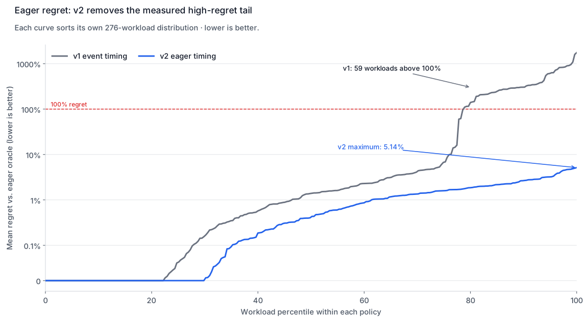
Figure 4. In this eager matrix, deployment-matched timing removes v1’s high-regret tail.

The matrix fixes $N=K=8192$ and varies $M$, token count, or batch size by operation. The 59 v1 workloads above 100% regret span bmm_fp8, mm_bf16, mm_fp4, and mla_decode. Of them, 57 have $M$ or batch size at most 64; the other two are mm_fp4 cases at $M=1024$.

Regret expresses relative cost; absolute latency shows the size of that cost on the measured calls. For each workload, we averaged avoidable latency across the three selection seeds. Across the 59, the median was 91.9 µs and the maximum was 270.7 µs. Figure 5 groups every one of those workloads by operation; the four rows are the complete set of operation surfaces represented in the high-regret tail. Each dot is one workload mean, the gray bar is the interquartile range, the black diamond is the operation median, and the blue line is the overall median. Their concentration at small $M$ matches the decode-oriented, host-sensitive regime in which the timing boundary matters most.

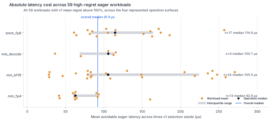
Figure 5. Absolute latency cost across 59 high-regret eager workloads.

These results measure tactic selection, not end-to-end serving. Translating them to request latency or throughput requires weighting each operation by how often it runs and how much of a request it occupies.

CUDA Graph execution: similar quality with a smaller regret tail

CUDA Graph replay provides a useful control regime. Here both policies already approximate the deployed work, so we expect a much smaller difference. Across 281 matched workloads, median regret fell from 0.0565% to 0.00646%, mean regret from 0.346% to 0.215%, the 90th percentile from 0.946% to 0.683%, and the count above 1% regret from 27 to 10. Both policies had the same maximum workload-level mean regret of 4.56%. Figure 6 summarizes the paired outcome for every workload.

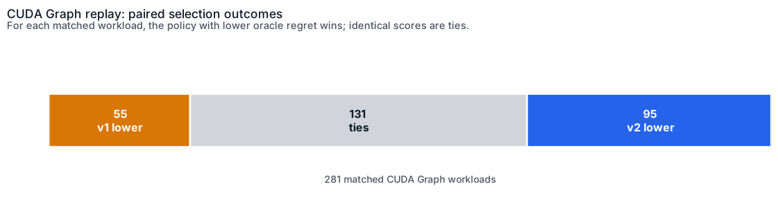
Figure 6. Under CUDA Graph replay, v2 had lower measured regret in 95 cells; v1 had lower regret in 55; 131 were tied.

The measured difference is modest, as expected when both policies already approximate graph replay. That contrast is the point: v2 reduces the smaller graph-regret tail without projecting the large eager mismatch onto graph-served paths.

Eager accuracy still matters in mixed-mode serving, including selected prefill, MLA, and distributed MoE paths. An engine can also request CUDA Graph measurement explicitly even when the surrounding warmup runs eagerly, so the tuning objective need not be inferred from the warmup context.

Persistence cost: pay at startup, not on every token

Persisting a correct winner is useful only if lookup does not add a recurring execution cost. Store attachment performs storage-dependent reads during warmup, so we separate that setup from first-touch and steady-state lookup latency.

Across B200 and GB300, with either the full runner list or only the winner, the four v2/v1 median dispatch-latency ratios ranged from 0.997 to 1.007, keeping v2 within 0.72% of v1. An audit recorded zero filesystem operations and zero JSON calls over 600 steady-state lookups.

The lookup measurements show where the one-time in-process work ends:

Lifecycle stage	Observed cost
First lookup and hydration	52.8–137.2 µs
Steady-state lookup	9.2–11.8 µs
Steady-state I/O audit	0 filesystem operations and 0 JSON calls over 600 lookups

Figure 7 shows all four measured configurations and their min-to-max ranges. The first lookup builds the key, resolves the winner, and promotes it into memory; subsequent lookups use the in-process winner.

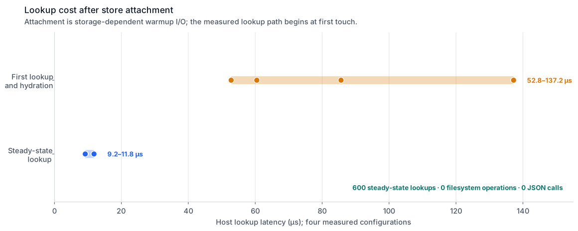
Figure 7. After first-touch hydration, lookup settles into the measured steady-state range.

Fresh-cache tuning cost was also close: across 24 GPU-by-operation pairs on B200 and GB300, the median v2/v1 wall-time ratio was 1.007, with v2’s default path included among its candidates.

Cache correctness under failure

Latency parity shows that reuse is cheap, not that it behaves correctly. Four groups of tests exercised distinct failure boundaries:

Test boundary	Observed result
Cold-to-warm reuse	A fresh process loaded the same keys and tactics; the warm restart triggered 0 new profiling starts.
Isolation and fail-closed behavior	Across 20 asserted controls, compatible stores hit as expected; cross-GPU, policy-mismatched, corrupted, and misplaced entries produced 0 wrong hits.
Key sensitivity	Each of 11 one-field perturbations changed the key.
Concurrent publication and reload	Four writers left 12 parseable entries and no temporary files; a separate reload discarded 7 unpublished local winners as designed.

Figure 8 places these checks beside the selection matrix. Each matrix cell reports eager / CUDA Graph matched-workload counts for one operation surface on one GPU; for example, 8/8 means eight eager and eight CUDA Graph workloads, not a quality score. A dash means that pair was not tested. The right-hand panel reports whether the restart, concurrent-write, reload, key-sensitivity, and isolation checks passed.

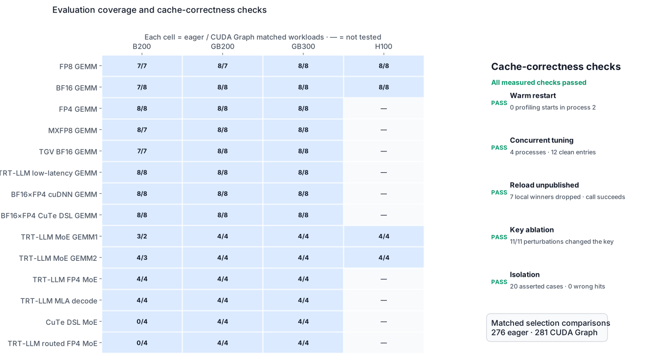
Figure 8. Measured operation coverage and cache-correctness checks.

Together, these tests cover the path from publication to reuse without claiming behavior outside the measured cases.

Rank agreement across distributed execution

Timing noise can make ranks select different tactics. For some distributed kernels, a tactic also determines how much NCCL-registered symmetric memory a rank allocates. Different rank-local choices can then create incompatible collective state and deadlock in tensor-parallel MoE serving.

Ranks can be made to agree at two points, and FlashInfer supports both:

On the measurements. The existing process-group reduction averages each candidate’s measured time across ranks. Every rank therefore selects from the same reduced measurements and arrives at the same winner.

On the result. Autotuner v2’s autotune_v2_reload() lets ranks tune concurrently, cross a framework-owned barrier, clear their local winners, and reload the final valid entry from the shared store.

The two paths need not choose the same tactic. Reduction selects the lowest mean measured time across participating ranks, at the cost of coordinating candidate measurements. Reload adopts the last valid published entry: it guarantees agreement, not a globally averaged optimum, and lets ranks tune independently until the barrier.

Use reduction when ranks can coordinate throughout profiling and the tuning objective should combine their measured times. Use reload when ranks must tune concurrently but can share a store and synchronize before serving. The mechanisms can also be combined: reduction aligns the in-session choice, while reload finalizes the persisted state.

We tested both paths on four GB200 ranks with deliberately noisy settings:

Coordination path	Observed keys	Keys with rank divergence
None	7	7
Reduced measurements	4	0
Barrier and reload	4	0

Figure 9 schematically contrasts the divergent control with the two protected paths; the counts come from the four-rank test.

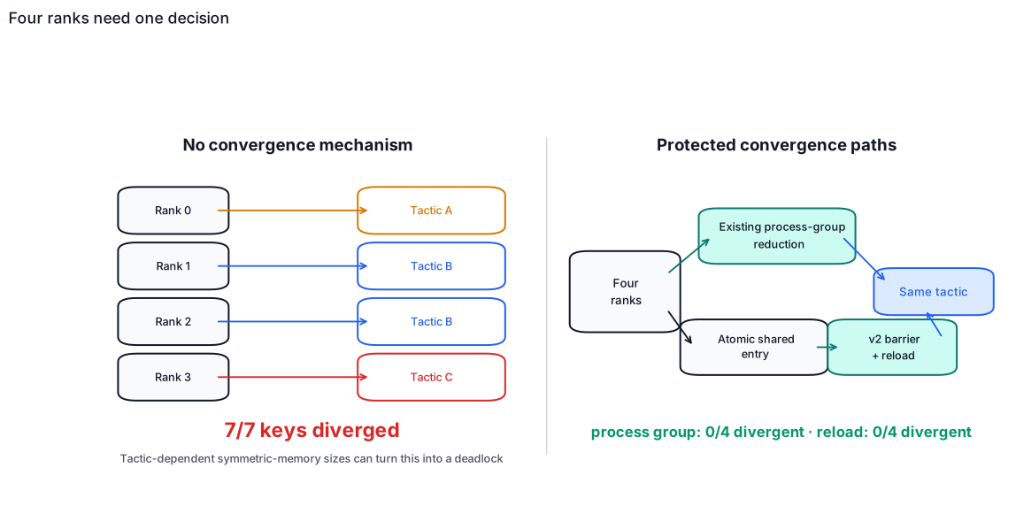
Figure 9. Both protected paths converged on every tested GB200 key.

What the measurements changed

The evaluation did more than score v2. It exposed avoidable lookup work, an incomplete persistent key, and setup work inside a diagnostic timing window. Each finding led to an implementation change.

Persistence measurements simplified the hot path. Profiling traced avoidable lookup work to repeated construction of nested key strings and runner keys after the winner was already known. Moving string construction out of the hot path and promoting decoded entries into memory produced the steady-state parity shown in Figure 7.

A key audit strengthened persistent identity. The SM100 MoE runner’s persisted key initially omitted constructor-fixed fields such as activation, weight layout, quantization, and expert structure, so two same-shape configurations could address the same entry. We added the relevant fields to that runner, completed the CuTe DSL MoE key with its missing expert and execution settings, and added input/output dtypes to the GEMM key. A separate GB200 ablation then perturbed 11 fields one at a time; all 11 changed the generated key, including top_k through runner extras.

Timer validation separated preparation from measurement. A cold-L2 probe fills a buffer so the next candidate does not inherit a warm cache. That preparation launches a 100–120 µs fill kernel, so v2 now completes and synchronizes it before opening the diagnostic timing window.

The timer audit also showed why CUPTI, NVIDIA’s profiling interface, is diagnostic here rather than the eager selection metric. For an eager moe_cute_dsl sequence of five Python-issued kernels, its GPU-side span was roughly 87% idle time between launches. CUPTI can show that the GPU is waiting between launches, but it does not capture the full wall-clock latency that an eager serving call pays. Across eight workloads and three seeds, CUPTI split 24 choices 13 to 11 between the 128- and 256-tile families, while graph-captured rescoring favored the 128 family on all eight workloads. We retain those eight workload cells in the aggregate but label them with this caveat. Figure 10 shows the mismatch.

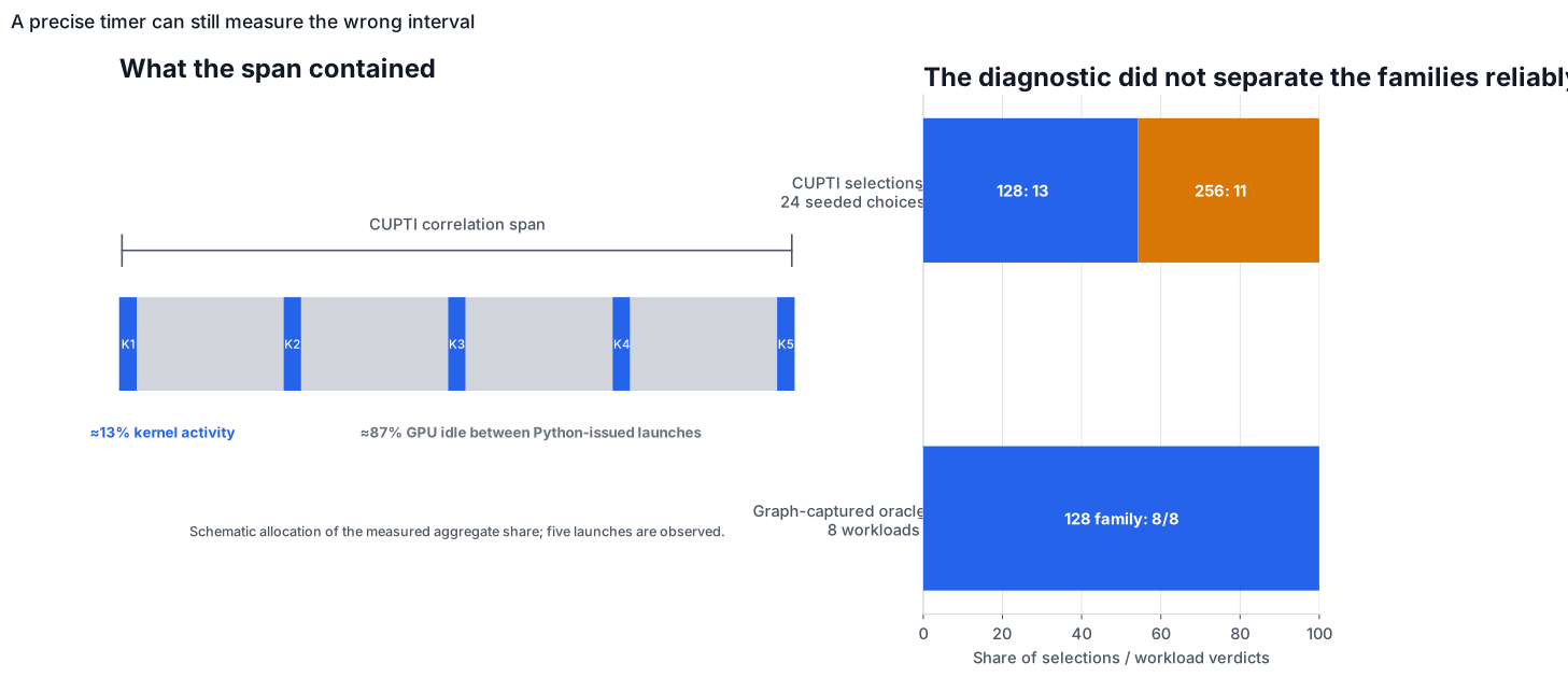
Figure 10. CUPTI captured mostly idle time for this eager MoE sequence.

The benchmark campaign therefore changed three implementation layers: the lookup hot path, persistent identity, and diagnostic timing.

Conclusion: tune the way you serve

Scaling kernel autotuning from a warmup measurement into a production serving system creates three coupled problems: measurement, artifact validity, and, in distributed execution, rank agreement.

Autotuner v2 connects those pieces around one rule: tune the path production will run. The measurement policy defines the timing boundary. Environment and operation identities define where a result can be reused. Autotuner v2 includes the default path among the candidates, publishes entries atomically, validates them where runners provide hooks, promotes decoded winners into memory, and provides explicit convergence paths.

The evaluation covers the same four questions. The eager results show the cost of measuring the wrong path. The smaller CUDA Graph result shows only a modest difference when both policies already measure similar work. The cache results show that stronger reuse checks need not become a per-token tax. The same evidence simplified the hot path, strengthened cache identity, and refined diagnostic timing.

The broader lesson is that the best tactic for serving is not determined by kernel time alone. It emerges from the kernel, launch path, capture mode, cache state, and the runtime around them. As inference stacks become more heterogeneous, autotuning must measure that context and preserve enough of its identity to know when a result remains valid.

Autotuner v2 is part of FlashInfer. The implementation and design history are available in PR #3861 and RFC #3920.

In future posts, we will share more of what we learn from measuring and deploying the low-level operators behind LLM inference. Stay tuned, and join the discussion in the FlashInfer project.

Acknowledgements

FlashInfer Autotuner v2 grew out of a substantial engineering effort within NVIDIA’s FlashInfer team, guided by systematic measurement and validation. As part of the broader FlashInfer community, we are building an open community around autotuning to advance GPU kernel selection for production LLM inference. We welcome contributions from ML systems researchers and practitioners.

We thank Yang Xu (NVIDIA; Senior Manager, FlashInfer and cuDNN) for driving the design, core implementation, and technical iteration of this effort; Albert Cheng (NVIDIA; Engineer, LLM Training and Inference) for system design, benchmark methodology, validation design, incorporating vLLM requirements, iterative development, and leading the drafting and writing of this article; Vincent Tombari (NVIDIA; Engineer, FlashInfer and cuDNN) for shaping the benchmarking methodology, collecting and validating measurements, developing and iterating on the evaluation, and providing extensive feedback on the article draft; Alex Yang and Brian K. Ryu (NVIDIA; Technical Leads, FlashInfer) for technical direction, design review, and extensive feedback on the article draft; Jingfan Sun (NVIDIA; Senior Manager, FlashInfer and cuDNN) for engineering leadership and project guidance; Lee Nau (NVIDIA; Engineer, SGLang) for iterative design feedback, SGLang requirements, and integration guidance; Xin Li (NVIDIA; vLLM Engineering Lead) for vLLM framework leadership and integration guidance; and Po-Han Huang (NVIDIA; SGLang Engineering Lead) for SGLang framework leadership and integration guidance. We are also grateful to the broader FlashInfer, vLLM, SGLang, and TensorRT-LLM communities for helping shape this work.

Citation

Please cite this work as:

Yang Xu, Albert Cheng, Vincent Tombari, Alex Yang, Brian K. Ryu, Jingfan Sun, Lee Nau, Xin Li, Po-Han Huang, and NVIDIA, “FlashInfer Autotuner v2: Tune the Way You Serve,” FlashInfer Blog, September 2026.

Or use the BibTeX citation:

@article{xu2026flashinferautotuner,
  author = {Yang Xu and Albert Cheng and Vincent Tombari and Alex Yang and Brian K. Ryu and Jingfan Sun and Lee Nau and Xin Li and Po-Han Huang and {{NVIDIA}}},
  title = {{FlashInfer} Autotuner v2: Tune the Way You Serve},
  journal = {FlashInfer Blog},
  year = {2026},
  month = sep,
  note = {https://flashinfer.ai/2026/09/22/autotuner-v2.html}
}